The optimal prediction problem
The starting point for the stochastic approach is a distribution of \(n\) price relatives between period 0 and period \(t\), with the price relative for good \(i\) given by \(p_{it} / p_{i0}\), for the population (universe) of all \(n\) goods and services to be measured by the price index. Associated with each good \(i\) is the probability \(P_{i}\) of observing this good transacted over both periods in the population of goods measured by the index, and this in turn gives a measure of frequency for observing different values for changes in price over time. Put differently, a price relative \(p_{t} / p_{0}\) is treated as a random variable in the stochastic approach, the distribution of which depends on the underlying distribution of goods and services that form the scope of the price index.22
Given a distribution of price relatives, the best predictor of a change in price between period 0 and period \(t\) is the value \(I^{A}\) that minimizes the expected prediction error. Formally, the best predictor solves the following problem23 \[\begin{align*} \min_{I} E\left[\left(\frac{p_{t}}{p_{0}} - I \right)^{2}\right], \end{align*}\] where \(E\) is the expected value operator, taken over the distribution of price relative. As is well known, the solution to this problem is to set \(I^{A} = E(p_{t} / p_{0})\) (Lehmann and Casella 1998, chap. 1 Example 7.17); that is, the best predictor of a change in price between two periods is the expected change in price. While it may seem unusual to express a price index in terms of an expected value, this simply emphasizes that a price index is rightfully a feature of the distribution of prices in the population. This is a key feature of the stochastic approach, and is what allows for a meaningful analysis of the statistical properties of a price index when calculated with a sample of price data from the population.
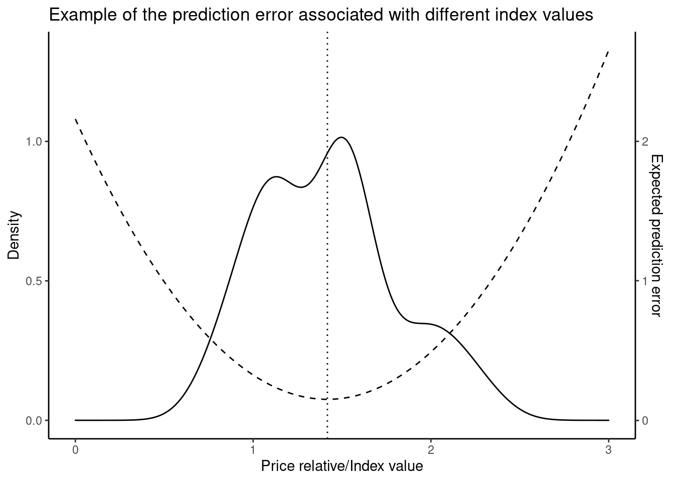
The figure gives an example of what the prediction problem looks like. Given a distribution of price relatives (solid line), there is an associated expected prediction error with each value that a price index can take (dashed line). The best choice for a price index as a predictive tool is the value that minimizes the expected prediction error (dotted line).
As the expected value is just a weighted average, the index \(I^{A} = E(p_{t} / p_{0})\) is simply an arithmetic index that averages price relatives. What’s interesting is that the weights now have a new interpretation—they are the probability of observing a good or service transacted in the population. That is, \[\begin{align*} I^{A} = \sum_{i = 1}^{n} \frac{p_{it}}{p_{i0}} P_{i}. \end{align*}\] Different arithmetic price-index formulas—e.g., Laspeyres, Paasche, Lowe—thus correspond to different statements about what determines the probability of observing a transaction. For example, with a Laspeyres index the probabilities are given by period-0 expenditure or revenue shares. This amounts to a statement that the probability of observing a transaction for a good is the likelihood of spending or receiving a dollar on that good in period 0.24
There is a tendency to think of this distribution as being Gaussian, but doing so means that some goods and services have negative prices. In most cases price relatives cannot be distributed Gaussian.↩︎
This is a prediction problem using a quadratic loss function, to ensure that the prediction error is always positive, and to formalize the idea that a large misprediction is more costly than many small mispredictions. Different loss functions usually give different optimal predictors; for example, the absolute loss function returns the median as the best predictor, which finds applications for housing price indices. If price relatives are symmetrically distributed, then all symmetric, convex loss functions give the same price index (Lehmann and Casella 1998, chap. 1 Corollary 7.19).↩︎
Selvanathan and Rao (1994, chap. 3) give an alternate interpretation: different index-number formulas come from different statements about the variance structure of price relatives and the use of inverse-variance weights to produce efficient estimators of inflation.↩︎