Sub-indices and aggregation
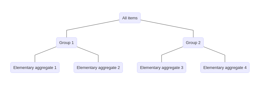
Most price indices have a hierarchical (or aggregated) structure, so that goods and services are partitioned into increasingly broad groups or categories that build up to all goods and services covered by the price index. For example, the goods in a CPI can be partitioned into broad categories such as food, shelter, transportation, etc. These categories are then broken into smaller categories; food may be partitioned into meat, diary, poultry, etc. This type of structure has the obvious benefit of providing a price index for sub-categories of goods and services that are often of interest in their own right (although there are other, more subtle reasons for wanting to structure a price index like this). The chart below gives an example of a simple aggregation structure with three levels.
A hierarchical structure does not pose any special challenges for making a price index—one of the index-number formulas from the previous section can always be used to aggregate the price relatives for the goods and services in each group of the hierarchy to produce a collection of price indices for each level in the hierarchy. The index calculation simply needs to be repeated for each group of goods and services in the aggregation structure. This is the direct approach to calculating a price index with a hierarchical structure.
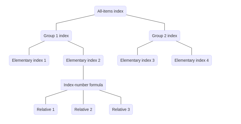
Having a hierarchical structure, however, suggests that the calculation can be simplified with a two-step procedure. In the first step, price relatives are combined at the lowest level of aggregation using one of the index-number formulas from the previous section. This gives a collection of price indices called elementary (or elemental) indices. These price indices give the movement in price over time for small, relatively homogeneous groups of goods and services called elementary aggregates that form the basis of a price index. Once the elementary indices have been calculated, indices for higher levels of aggregation are calculated by combining elementary indices using weights. These weights provide a measure of the economic importance of the goods and services in each elementary aggregate in order to combine elementary indices together to form a higher-level index. If the target index is an arithmetic index, then the elementary aggregates should be combined with a weighted arithmetic average; otherwise, if a geometric index is the target index, a weighted geometric averaged should be used. Put differently, each elementary aggregate is treated as a single good, with the elementary indices being the price relatives for these goods, and this information is fed into an index-number formula to produce a higher-level index.
Given that there are two ways to calculate a price index with a hierarchical structure, does the direct calculation give the same result as the two-step calculation? The answer is yes for an arithmetic or geometric index, provided the weights used to aggregate the elementary aggregates are formed using the underlying weights for the target index. For example, if the goal is to calculate a Laspeyres index, then the weight for an elementary aggregate should be the expenditure/revenue share for the goods in that elementary aggregate in period 0. As both geometric and arithmetic indices are calculated as weighted averages, it should not be surprising that an index can be calculated by first grouping price relatives together, calculating group-level averages, then averaging the group-level averages to form an overall average. Consequently, these indices are said to be consistent in aggregation, although not all index-number formulas are consistent in aggregation. For example, the Fisher index is not consistent in aggregation, and using the two-step procedure to calculate it will give a different answer than the direct calculation.
It is easy to show that any arithmetic index is consistent in aggregation (the reasoning for the geometric case is almost identical). Suppose that goods are partitioned into \(k=1,\ldots,m\) distinct and mutually exclusive categories—that is, there are \(m\) elementary aggregates. If category \(k\) contains \(n_{k}\) goods, then the arithmetic index for this category is \[\begin{align*} I_{k}^{A} = \sum_{i = 1}^{n_k} \frac{\omega_{ik}}{\sum_{j = 1}^{n_k} \omega_{jk}} \frac{p_{ik1}}{p_{ik0}}, \end{align*}\] where \(p_{ik1} / p_{ik0}\) is the price relative of good \(i\) in category \(k\) and \(\omega_{ik}\) is the weight for good \(i\) in category \(k\). These \(m\) indices can now be aggregated together to form an overall index by taking a weighted-average of each index, with weights given by \(\omega_{k} = \sum_{j = 1}^{n_k} \omega_{jk}\), so that \[\begin{align*} I^{A} &= \sum_{k = 1}^{m} \omega_k I_{k}^{A} \\ &= \sum_{k = 1}^{m} \omega_k \sum_{i = 1}^{n_k} \frac{\omega_{ik}}{\sum_{j = 1}^{n_k} \omega_{jk}} \frac{p_{ik1}}{p_{ik0}} \\ &= \sum_{k = 1}^{m} \sum_{i = 1}^{n_k} \omega_{ik} \frac{p_{ik1}}{p_{ik0}}. \end{align*}\] But this is exactly the same as if the arithmetic index had been calculated by pooling all price relatives together and calculating the index directly, rather than partitioning them into groups and calculating the index in two steps.
One advantage of the two-step calculation over the direct calculation is that the index-number formula used to calculate the elementary indices can differ from the index-number formula used at higher levels aggregation. It may seem odd to want to do this, but there are a number of subtle theoretical and practical reasons why a different index-number formula would be used for the elementary indices. In most applications the elementary indices are calculated using a Jevons index, partly because detailed information on quantities bought or sold may be difficult to obtain at very low levels of aggregation. Higher levels are then calculated as an arithmetic index, usually a Young or Lowe index.